Appearance
Cohorts: alignment and shape models
Correspondence through a shared structure
An encoding is a feature vector
(centerline control points, angular reference, section tilt coefficients
Branched vessels
A branched vessel is a tree of tubes, and its feature vector is that of every branch, each followed by its wall domain
The angular origin of a child is carried over from its parent at the junction by the smallest rotation that takes the parent's tangent to the child's (see Sections of a branch), so
A shared structure
encode_cohort enforces a shared structure:
- Tree. Every subject is encoded first as it would be alone. Their trees must be the same; the encoding then keeps the reading of every subject's junctions.
- Sizes. Sizes given as rules are resolved for every subject, and the cohort uses the median, branch by branch.
- Domain. At the inlet and the outlets, every wall ends at the boundary centroids:
and at the free ends of every subject (end mode centroid). Where a branch meets a junction its domain is a feature. - Knots. With adaptive knots, the normalized variation profiles of all subjects (pilot fits on uniform knots) are averaged and a single knot vector is placed from the mean profile (Adaptive knots), for every branch; then all subjects are refitted on them.
Generalized Procrustes alignment
Feature vectors also contain position and orientation, which are usually irrelevant. Let alignment.tau_samples rings, shared among the branches in proportion to their mean length, with alignment.theta_samples points each). Generalized Procrustes analysis (Gower [11]) finds similarities
by alternating: (i) centre every alignment.tolerance times its RMS radius.
The similarity is then applied exactly to each encoding: control points transform as points, the reference direction rotates, the rotation-minimizing frame follows the centerline (it is equivariant under rotations), the tilt is relative to that frame and does not change, and wall coefficients scale by
Principal component analysis
With aligned feature vectors model.variance_fraction of the total variance, and represents shapes as
with
Decoding
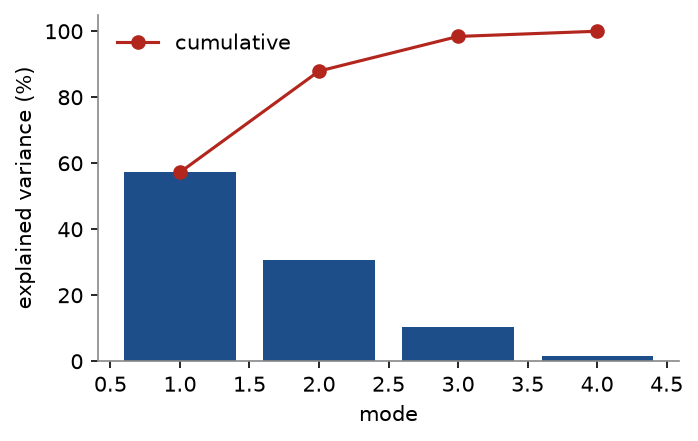
Explained variance of the synthetic cohort of the user guide: four parameters vary, four modes explain all the variance.
Meshes with the same faces
The walls of unbranched shapes are triangulated on their
- Every vertex keeps the branch that dominates it in the mean, the angle
of the nearest point of that branch's wall in its section, and its signed distance from that point, in radii of the branch (its wall coordinates). - Its
keeps its place relative to the anchors of the branch: the ends of its windows and of its wall domain, which differ from shape to shape. Between anchors is mapped linearly, beyond them it is shifted (along the extensions it is still a length). - Around the mouth of every side branch, where its centerline becomes fully present, the coordinates of the branch it leaves follow the mouth: they are shifted by the displacement of the mouth in that branch's
, weighted by a smooth step that falls from one at the mouth to zero three side-branch radii away. - The vertex is placed by the coordinates of its branch in the shape (at that distance along the normal of the section curve), and moved onto the shape's wall along the gradient of the union. Where the junctions of the two shapes differ most (in a crotch between close branches) some faces can fold; their vertices are moved to the mean of their neighbours and back onto the wall.
The result has the faces of the mean's mesh and lies on the shape's wall, except in small patches in the crotches between close branches (Validation). The furca model modes meshes and the shape views of the application are built this way, so that a shape can be animated by moving the vertices of one mesh.