Skip to content

Wall ​

Model ​

Every cross-section is a closed curve in the coordinates (x,y) of its plane (along the in-plane axes U, V of the section frame), parametrized by the harmonic angle φ. It is written in the frame that turns with φ,

W(τ,φ)=ρw(τ,φ)e(φ)+σw(τ,φ)e⊥(φ),e=(cos⁡φ,sin⁡φ),e⊥=(−sin⁡φ,cos⁡φ),

with a radial component ρw and a tangential component σw, both tensor-product cubic B-splines on the same bases,

ρw(τ,φ)=∑i=0nτ−1∑j=0nφ−1aijBi(τ−τaτb−τa)Pj(φ2π),σw(τ,φ)=∑i,jbijBi(⋅)Pj(⋅),

with Bi a clamped and Pj a periodic cubic basis (B-splines), over the domain [τa,τb] chosen as described in Ends. The wall is C2 everywhere, including across φ=0.

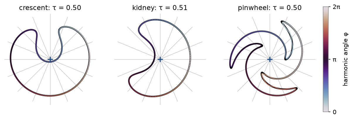
σw is how far the wall departs from the ray at its own angle. A star-shaped section parametrized by its polar angle has σw=0, and ρw is then its radius function: the model contains the radius-function wall as the case σw=0, φ=θ, which wall.angle = "polar" selects. On a section that is not star-shaped about the centerline, the wall turns back on itself as seen from it, and σw carries it there.
Encoded cross-sections that are not star-shaped

Cross-sections of the three synthetic tubes that are not star-shaped (black: exact; colour: encoded, by the harmonic angle φ), with rays from the centerline (grey) that meet the wall more than once.

The components are written in the turning frame rather than as (x,y) themselves for two reasons. The bending energy below vanishes on a circle about the centerline parametrized by its angle, as that of a radius function does, while the second derivative of x and y around a circle does not: penalizing it would pull every section towards a point. And holes in the data (the mouth of a side branch) are filled with a round wall, not drawn towards their chord (Branched vessels).

Fit ​

Every wall vertex pk has its section τk and its coordinates (xk,yk) in that plane (vessel coordinates), its harmonic angle φk and a weight wk equal to its barycentric area Ak=13∑T∋k|T|, normalized to mean one. Area weights make the fit approximate a surface integral, so the result does not depend on local mesh density.

The squared distance between the vertex and the wall at its angle is the same in the frame that turns with φk, where the vertex has the components rk=(xk,yk)⋅e(φk) and sk=(xk,yk)⋅e⊥(φk):

|(xk,yk)−W(τk,φk)|2=(rk−ρw(τk,φk))2+(sk−σw(τk,φk))2.

The fit therefore splits into two independent scalar fits with the same design, weights and normal matrix: one factorization serves both, and the smoothing is chosen for both together.

The coefficients minimize the penalized least squares objective with the bending energy of both components in physical units as penalty:

J=∑c∈{ρw,σw}∬(∂2c∂s2)2+(∂2c∂ℓ2)2dsdℓ,

where s is arc length along the vessel and ℓ=r¯φ arc length around it. Writing t∈[0,1] and u=φ/2π for the basis parameters, Ld for the physical length of the domain and C=2πr¯ for the mean circumference, and using ∂s=Ld−1∂t, ∂ℓ=C−1∂u,

J=∑cc⊤(CLd3Ωt⊗Mu+LdC3Mt⊗Ωu)c∝∑cc⊤(Ωt⊗MuLd4+Mt⊗ΩuC4)c,

with Mij=∫01BiBj and Ωij=∫01Bi″Bj″ computed exactly by Gauss–Legendre quadrature on each knot span (the O'Sullivan penalty [9]). The penalty is isotropic in physical space, so a single smoothing parameter λ, chosen by GCV, suffices whatever the length, radius and knot placement. Unlike difference penalties, it remains correct for non-uniform knots. With two components, GCV minimizes NRSS/(N−edf)2 with the residual sum of squares of both.

Parameter correction ​

The discrete harmonic angle carries tangential noise of the order of the irregularity of the mesh. Fitted as it is, that noise counts as misfit, and GCV answers it with more smoothing than the wall needs. After the first fit, every vertex therefore takes the angle φk∗ of its nearest point on the fitted wall in its section, and the wall is fitted again (wall.corrections times; one by default). This is the parameter correction of curve fitting (Hoschek [28]): the angles keep the smooth part of the harmonic angle and lose its noise. On the synthetic tubes one correction brings the error of the circular and elliptic presets to that of a radius function fitted on the polar angle.

The nearest point is found by sampling the section at four points per coefficient (the values of a uniform periodic basis repeat from span to span, so the samples cost a few operations each) and refining the nearest sample by Newton's method on the stationarity of the squared distance.

Adaptive knots ​

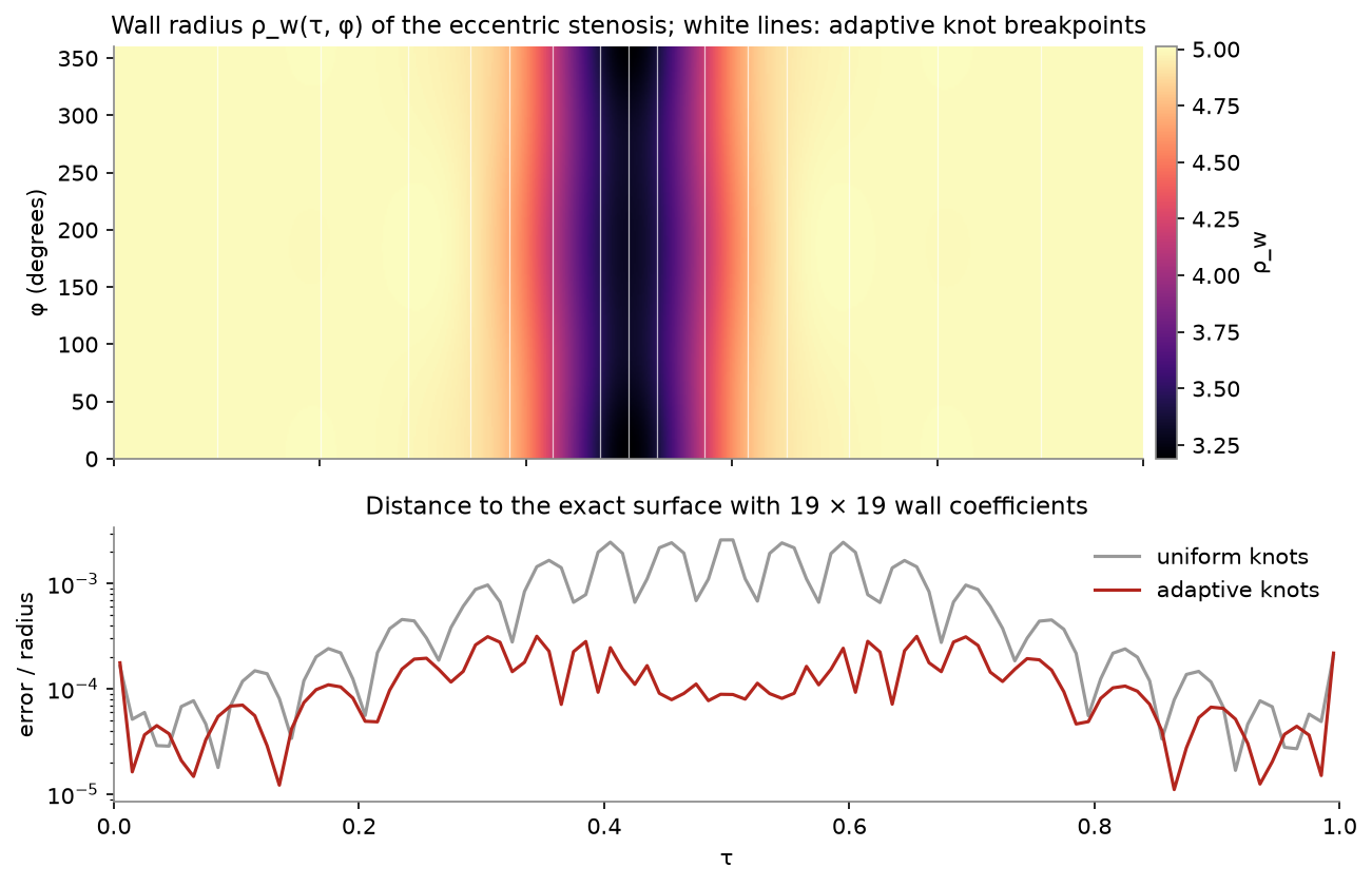
Vessels are not uniformly complex along their length: a stenosis or an aneurysm neck needs more resolution than a straight segment. With wall.knots.mode = "adaptive" (the default) the longitudinal knots are placed in two passes:

  1. Fit the wall on uniform knots.
  2. Compute the angular RMS of the longitudinal curvature of the wall, g(t)=(12π∫|∂t2W|2dφ)1/2 (exactly, as ∑ca⊤Mua with aj=∑iBi″(t)cij for both components), on samples_per_span points per span.
  3. Form the knot densityd(t)=(1−α)+αg(t)1/2g1/2―,α=strength∈[0,1),and place the interior knots at equal quantiles of ∫0td.
  4. Refit on these knots.
Wall radius map with adaptive knots and error profile

Top: the wall radius of the eccentric stenosis, unrolled; vertical lines are the adaptive breakpoints, concentrated around the throat. Bottom: distance to the exact surface along the vessel with the same 19 × 19 coefficients for uniform and adaptive knots.

The exponent ½ follows the classical result that the error of spline approximation is equidistributed when the local knot spacing h satisfies h2|f″|≈ const (de Boor [10]). The uniform share 1−α keeps knots everywhere so that the second fit can still represent features the pilot missed; on the test cases α=0.5 is best and stronger concentration (α=0.8) is worse. For a stenosis at a fixed budget of 19×19 wall coefficients, adaptive knots reduce the mean error fourfold (see Validation). When the wall varies uniformly the density is constant and the knots stay uniform.

Each observation touches 4×4 coefficients, so B⊤WB is block banded: it is accumulated as nτ×4 blocks of size nφ×nφ, in parallel over fixed-size chunks of samples combined in a fixed order.

Section measures ​

The area of a section, 12∮(xdy−ydx), and its perimeter are integrated exactly in φ (3-point Gauss–Legendre on every span); the equivalent radiusA/π replaces the angular mean of a radius function. The distance from the centerline to the wall, |W|, is still the wall radius where the section is star-shaped.

Reported diagnostics ​

The encoder reports the residuals, the distance in its section plane from every vertex to the encoded section (mean, RMS, 95th percentile, maximum), the chosen λ, the effective degrees of freedom, the extensions beyond the centerline ends, the number of excluded vertices, and the fraction of the sections that are not star-shaped about the centerline (non_star_fraction: those whose polar angle does not increase with φ all around). furca evaluate computes true point-to-surface distances.

furca — parametric models of blood vessels.